How To Add Formula In Excel Chart
Add or remove series lines drop lines high-low lines or. Go to the formula bar and type.

How To Add Trendline In Excel Charts Myexcelonline Microsoft Excel Tutorial Excel Tutorials Chart
For our example type 11.

How to add formula in excel chart. Right-click the chart and then choose Select Data. 2 days agoTo create an Organization Chart in Excel follow the steps below. Here are the steps.
Its even quicker if you copy another series formula select the chart area click in the formula bar paste and edit. Select the data you want to represent in graph. Select the chart label you want to change In the formula bar hit equals and select the cell reference that contains the data for your chart label.
Highlight Distinct Values in Excel 365. How to Quickly Create a Gantt Chart in Excel 365 Step by Step. Select the cell which you want to link with chart title.
The textbox will always display the text in Sheet1A1. Click SmartArt in the Illustration group. The first conditions checks to see if the column date is greater than or equal to the start date.
Highlight Rows Between Two Strings in Excel 365 Formula Rules. Leaving the dialog box open click in the worksheet and then click and drag to select all the data you want to use for the chart including the new data series. We now need to create a chart based on the values in cells A8-M9.
Add to formula with shortcut. Select the chart area of a chart click in the Formula Bar or not Excel will assume youre typing a SERIES formula and start typing. In the Choose a SmartArt gallery select Hierarchy.
For stopping this changing you need to add to the cell reference and change the relative reference to absolute reference. The formula instructs Excel to do the following. Select LinkedCell and enter the cell that you want to link it to.
Enter the data from the sample data table above. The Select Data Source dialog box appears on the worksheet that contains the source data for the chart. Click on the Column chart drop down button.
Insert a textbox in the chart and with the textbox selected write in the formula bar a formula that refers to a cell like. On the worksheet click the cell in which you want to enter the formula. If you change the name in cell A9 the formulas will update to display the figures for the new name.
Click the Insert tab. Then right click on the text box to see properties. Cell References and Arrays in the SERIES Formula.
Specific line and bar types are available in 2-D stacked bar and column charts line charts pie of pie and bar of pie charts area charts and stock chartsPredefined line and bar types that you can add to a chartDepending on the chart type that you use you can add one of the following lines or bars. Note that the formula in cells B9-M9 uses the Excel Column and the Excel Vlookup functions to look up the data for the name in cell A9. Copy the formula from cell B9 into cells C9-M9.
Click on INSERT tab from the ribbon. To get the desired chart you have to follow the following steps. Type the equal sign followed by the constants and operators up to 8192 characters that you want to use in the calculation.
The second condition checks that the column date is less than or equal to the end date. Your workbook should now look as follows. From the Developer tab on the ribbon select Controls Design Mode Insert then in the bottom half ActiveX select Text Box and create your text box.
If cell C2 is blank then return an empty string blank cell otherwise apply the cumulative total formula. For example you apply the formula is A1B1 in Cell C1 and it will change to F12G12 as you copy it to the Cell H12. How to Highlight the XLOOKUP Result Cell in Excel.
Select chart title in your chart. Go to the formula bar and type the equal sign into the formula bar then select the cell you want to link to the chart title. Welcome to the board.
By following this method you can addshow task names next to the Gantt Chart bars in Excel 365. The formula is based on the AND function configured with two conditions. Now you can copy the formula to as many cells as you want and the formula cells will look empty until you enter a number in the corresponding row in column C.
How To Copy Formulas In Excel Excel Excel Formula Formula

Excel Variance Charts Making Awesome Actual Vs Target Or Budget Graphs How To Pakaccountants Com Excel Tutorials Excel Shortcuts Excel

How To Create Interactive Excel Charts With The Index Formula Excel Charts Chart Excel

Excel Chart Of Top Bottom N Values Using Rank Function And Form Controls Pakaccountants Com Excel Tutorials Data Dashboard Excel Shortcuts

Understanding Excel Operators Guide Pakaccountants Com Business Analyst Tools Microsoft Excel Tutorial Excel Shortcuts
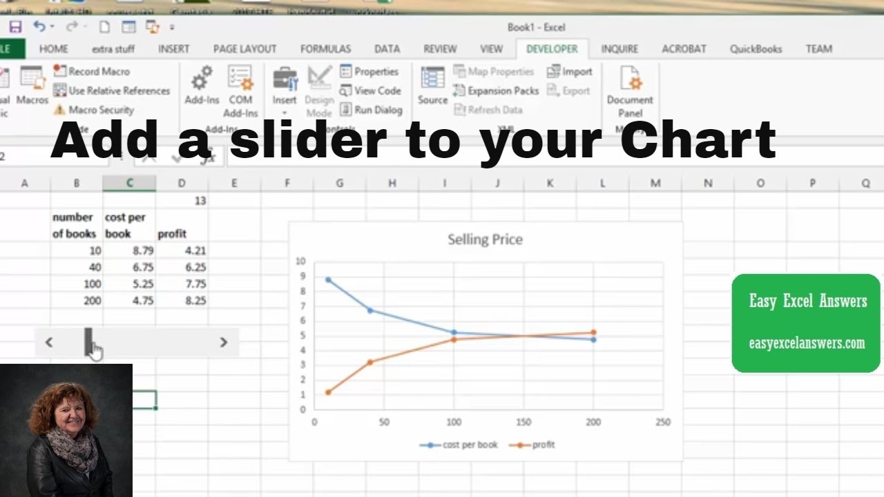
Add A Slider To Your Chart In Excel Excel Excel Shortcuts Job Information

Basic Microsoft Excel Formulas Cheat Sheets Keyboard Shortcut Keys Hacks Excel Formula Microsoft Excel Formulas Computer Shortcut Keys

Follow These Easy Steps To Create A Pivot Table In Microsoft Excel 2016 Excel Pivot Table Microsoft Excel Tutorial

How To Create Gauge Chart In Excel Free Templates Excel Microsoft Excel Formulas Gauges

Pin On Microsoft Office

How To Create Gauge Chart In Excel Free Templates Excel Excel Templates Microsoft Excel Formulas

How To Create A 2d Clustered Column Chart In Microsoft Excel Microsoft Excel Chart Excel

Excel Variance Charts Making Awesome Actual Vs Target Or Budget Graphs How To Pakaccountants Com Excel Shortcuts Microsoft Excel Formulas Excel

Count Sum Cells Based On Cell Colour In Excel How To Pakaccountants Com Microsoft Excel Tutorial Excel Tutorials Excel

Spreadsheet Page Excel Tips Creating A Thermometer Style Chart Excel Shortcuts Excel Tutorials Excel Spreadsheets

Ultimate Dashboard Tools For Excel Advanced Chart Add In Dashboard Tools Excel Dashboard Templates Excel

Excel Magic Trick 267 Percentage Change Formula Chart Youtube Microsoft Excel Tutorial Excel Tutorials Formula Chart

How To Create A Waffle Chart In Excel Excel Chart Microsoft Excel
